The Yasuyo building, Shinjuku, March 2025
Introduction
The issue of how to analyse data on repeated observations on the same units over time (i.e. panel data/longitudinal data) occurs frequently. For example, visitors returning to a website, the prices of a group of houses over time, people’s pattern of TV viewing and survey respondents answers to repeated questions on their self-assessed well-being (scored between 1 and 10) to name just a few examples I’ve encountered.
The below are some notes to refresh my knowledge of the basics of the topic. What follows assumes some knowledge of regression and linear algebra. It is based on the treatment of the topic in Davidson & Mackinnon and Johnston & DiNardo.
Panel data and the estimation issues it creates
We assume there are T observations over time on m different units. The dependent variable is represented by y an (m x T, 1) vector, the n explanatory variables X are a matrix of dimensions (m x T, n) and we are estimating a vector β of n coefficients. We represent this with a corresponding error term as:

The error for unit i at time t consists of a unit specific effect η_i and a time specific unit effect ε_it.
 The standard Ordinary Least Squares (OLS) estimator for this is:
 This gives y_hat the predicted value of y for a given X.
 A geometric interpretation of this is that y_hat is the projection of y onto the space spanned by vectors that are the explanatory variables X. Where y_hat is determined by the vector of coefficients β that minimise the difference (the sum of squared errors) between y and y_hat.
If we estimate a regression on panel data using a standard OLS estimator as if we have m x T independent observations, rather than T repeated observations on the same m units, then this can create problems:
-Biased estimates of the coefficients from omitted variable bias Running a regression, without adjusting for the fact that repeated observations come from the same units, is likely to cause a form of omitted variable bias. This is because it is quite probable that there are unit specific effects that affect the dependent variable which are not fully captured by the explanatory variables. If these unit specific effects are correlated with the explanatory variables then this will result in the OLS estimates of their coefficients being biased.
-Inefficient estimates due to heteroscedasticity of errors Unit specific effects are highly likely to result in heteroscedasticity as each unit in the regression data will probably have unit specific errors, leading to errors being correlated across repeated observations on panel members. This is likely to generate inefficient estimates as in this context OLS is not making optimal use of its inputs: an additional observation on a unit in OLS is given the same weight as observations on a new unit even though the latter conveys more information.
Two standard approaches to estimating regressions on panel data to address these are now described:
- Fixed effects (which helps remove the bias)
- Random effects (which helps improve efficiency)
In what follows, we sometimes refer to the units as individuals or groups.
1. Fixed effects: Using the variation in the individual units over time (and removing the cross-sectional variation) to estimate the coefficients
In the simplest form of fixed effects estimation we assume that each unit’s identity has an effect on the dependent variable which does not vary over time e.g. if y is spending and X is a set of data on personal characteristics then person i will always spend η_i more (or less) depending on who they are.
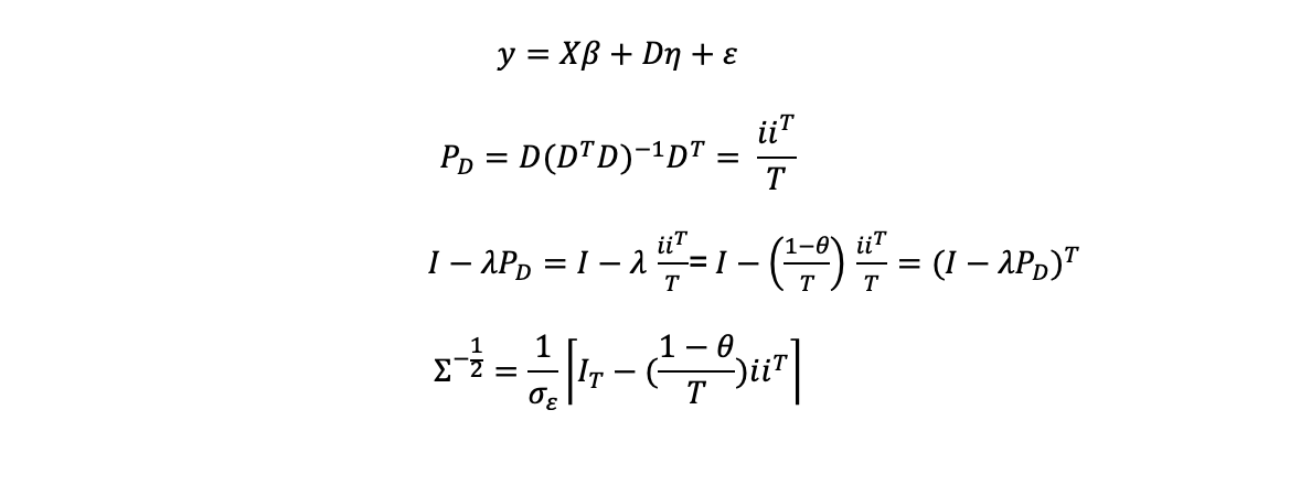
One way to adjust for these effects is by estimating the following equation where X are the explanatory variables, D is a set of dummy variables and η
is a vector of individual specific effects which do not vary over time. D is specified by an (m x T, m) matrix of group/individual specific dummies which is 1 for unit i’s data for all time periods, but which is otherwise zero.
 We do not necessarily need to estimate the regression using dummy variables to control for the fixed effects as there are other ways to adjust for them. A standard approach is to take the
dependent variable y and the variables in X and for each unit subtract the mean value for that unit for each variable. This has the benefit of not requiring as large a sample size as is needed
to estimate the individual fixed effects.
We do not necessarily need to estimate the regression using dummy variables to control for the fixed effects as there are other ways to adjust for them. A standard approach is to take the
dependent variable y and the variables in X and for each unit subtract the mean value for that unit for each variable. This has the benefit of not requiring as large a sample size as is needed
to estimate the individual fixed effects.
To see why this works we split a general regression’s explanatory variables into two sets X_1 and X_2 (We will later specialise to X_2 being the dummy variables that
describe when observations relate to a given unit).
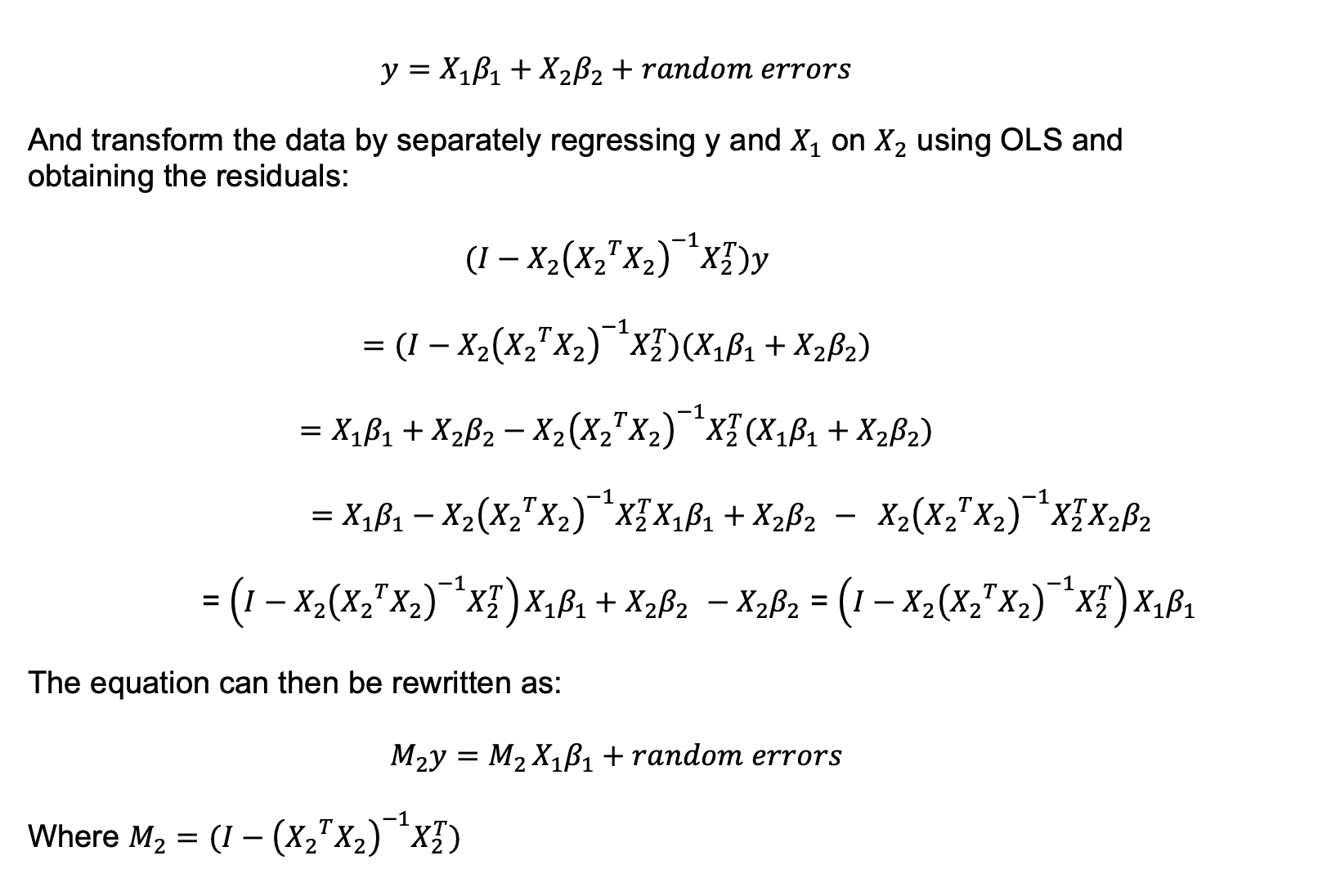 By regressing the measured y and the relationship with X_1 and X_2 on the other variables X_2 we obtain as residuals the variation of y and X_1 that cannot be explained by
variation in X_2. X_2 by definition accounts for its own variation perfectly and so drops out of the equation.
If we then estimate an OLS regression on this transformed y and X_1 data we can isolate the effects of the Betas for X_1.
By regressing the measured y and the relationship with X_1 and X_2 on the other variables X_2 we obtain as residuals the variation of y and X_1 that cannot be explained by
variation in X_2. X_2 by definition accounts for its own variation perfectly and so drops out of the equation.
If we then estimate an OLS regression on this transformed y and X_1 data we can isolate the effects of the Betas for X_1.
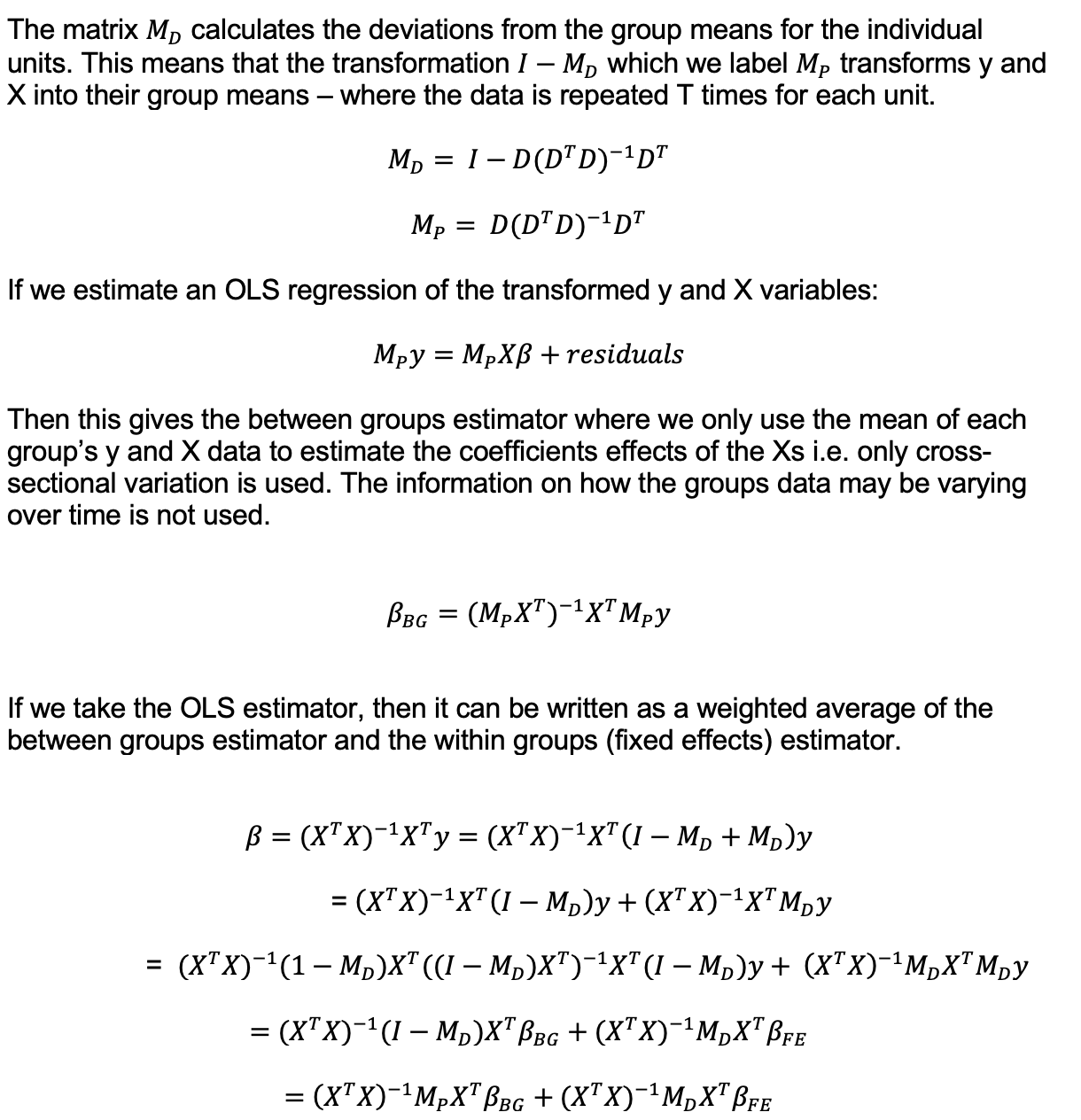
In the case of adjusting for the unit specific effects the X_2 variables are the dummy variables in the matrix D. These variables are 1 for a given unit across all time periods, but otherwise zero. As shown below, the resulting transformation M_D is equivalent to taking the dependent and explanatory variables and subtracting their unit level means.
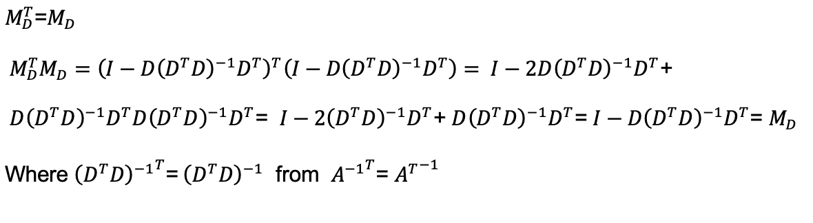
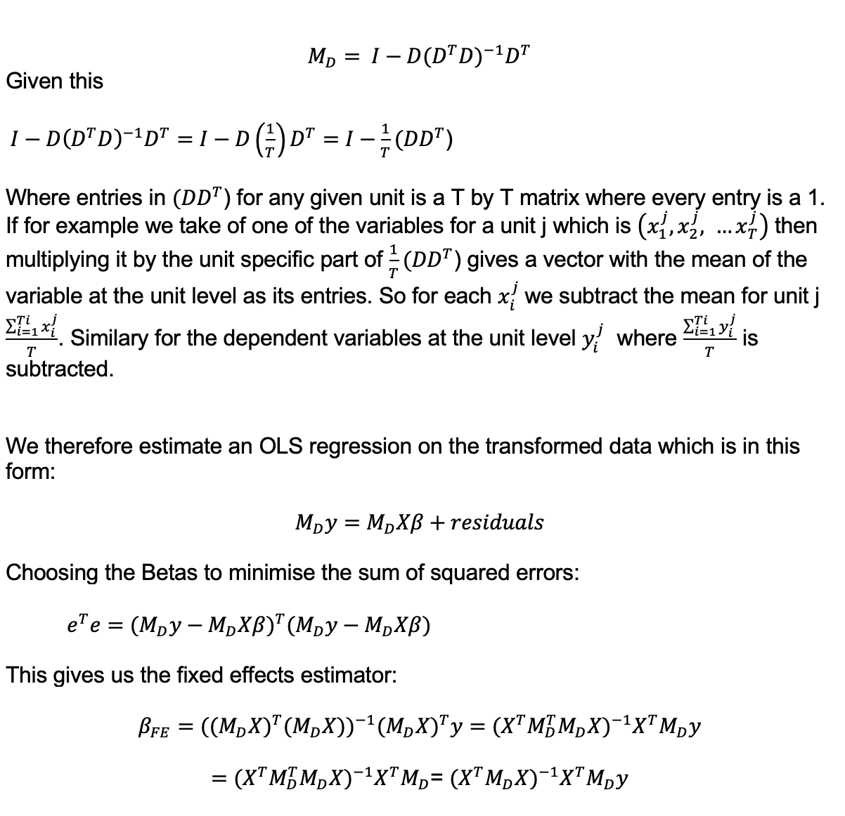 Where the following properties of M_D are used:
 A consquence of fixed effects estimation is that there will not be an overall constant term. Unit specific constants are set to zero by subtracting their means as the constant term will be fixed across all time periods so will not appear in the estimates. As a result although the fixed effects estimator gives coefficient estimates of the effects of the explanatory variables, it does not directly give a prediction of the level of the dependent variable.
We have shown that we can control for unit level specific effects on the estimated coefficients by subtracting the data’s unit level means. Only variation relative to a unit’s mean affects the estimate. The level of a unit’s data, its mean, relative to others does not matter. Fixed effects estimators are often referred to as within groups estimators as they only use the variation within groups. The opposite of this is the between groups estimator which is, for the same sample, a regression on the mean of each variable’s unit level values removing any time variation. As shown in Appendix 1 the OLS estimator is a mixture of within and between group estimates.
The advantages and disadvantages of fixed effects estimation
In most cases it is highly likely there will be factors that affect the outcome of the dependent variable we are interested in, but which we do not have information on e.g. people may have similar incomes and demographic characteristics, but spend quite different amounts of money on consumption. This could relate to differences in psychology, wealth, education or many other factors. We are though unlikely to have complete information on all the relevant factors. Fixed effects estimation offer us the potential to adjust for these differences even if we do not have data on them. As long as the unit specific effects do not vary over time we can remove their effects on the coefficients by using variation from the mean to estimate the regression.
As the errors from the fixed effects estimator are likely to be correlated across the repeated observations on units over time there will though be heteroscedasticity in the errors resulting in fixed effects estimators being less efficient i.e. having a higher variance.
Conceptually, although the ability of fixed effects to remove the time-invariant unit effects is attractive. It is also more sensitive to measurement error in the explanatory variables as it uses the variation over time in the variables which is likely to be more driven by this.
Another limitation is that the assumption of time-invariant fixed effects is probably not true in many cases of interest. A standard example of this is estimating the effect of a government training programme on a group of people. It may not be possible to observe data on it, but it is plausible that a factor which makes people want to participate in such a scheme is a change in their circumstances, but this by definition will not be a time-invariant fixed effect.
2. Random effects: Treating the unit specific effects as random variation and adjusting for the heteroscedasticity with Generalised Least Squares (GLS)
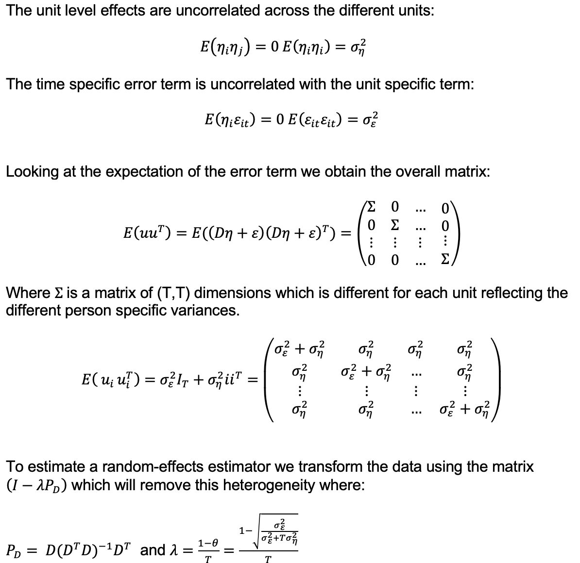
In the random effects model we treat the individual level effects as random variables. We therefore estimate a form of GLS which corrects the estimator for the heteroscedasticity caused by correlated errors at the unit level over time. In this instance we make a series of assumptions about the error terms:
 The variance parameters in the lambda are estimated using the variance of the:
-within groups regression errors to estimate the unit specific variance
-between groups regression errors to estimate the variance of errors across units
If there is no variation in unit specific effects then the effect is constant across units, lambda collapses to 0 and we revert to a standard OLS estimator. If we have a large enough set of observations over time T then we also converge on OLS as the variation in the unit specific effects tends to 0 with the larger sample. If lambda is 1 then the random effects estimator becomes the fixed effects estimator.
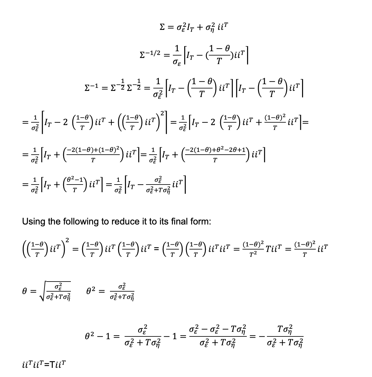
Where we have used:
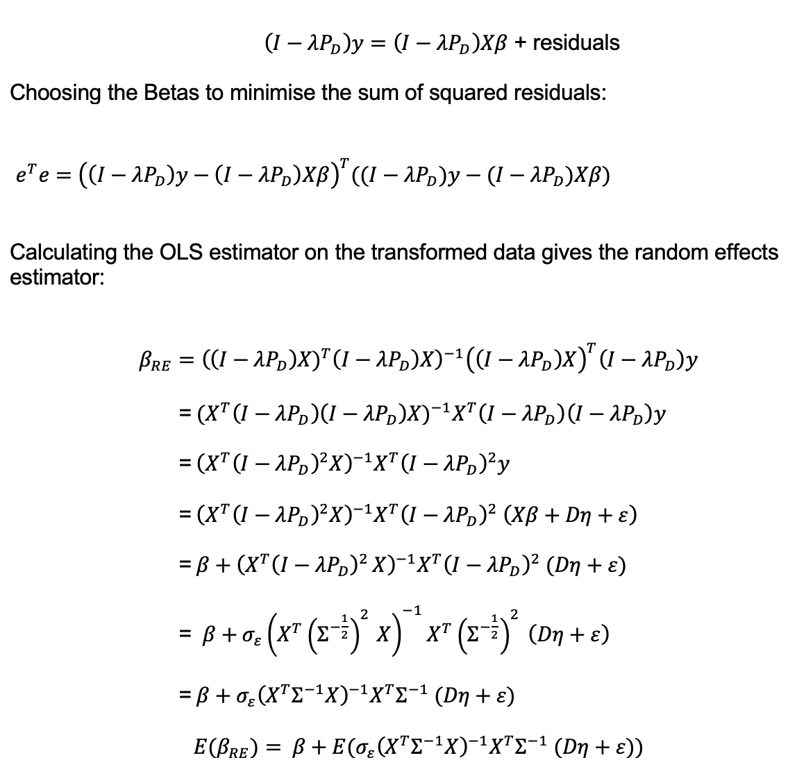
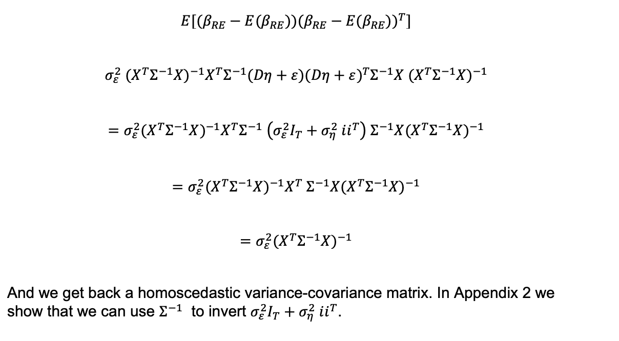
 Calculating the variance-covariance matrix:
The advantages and disadvantages of random effects estimation
If we look at the second-term of the expectation of the random effects estimator then we can see that if the unit specific effects are correlated with the explanatory variables the second-term
will be non-zero and therefore the GLS estimator biased. However, if this is not the case, the random effects estimator has an attractive property. The fixed effects, between
groups and standard OLS estimators can all be generalised to being special cases of the following weighted least squares estimator:
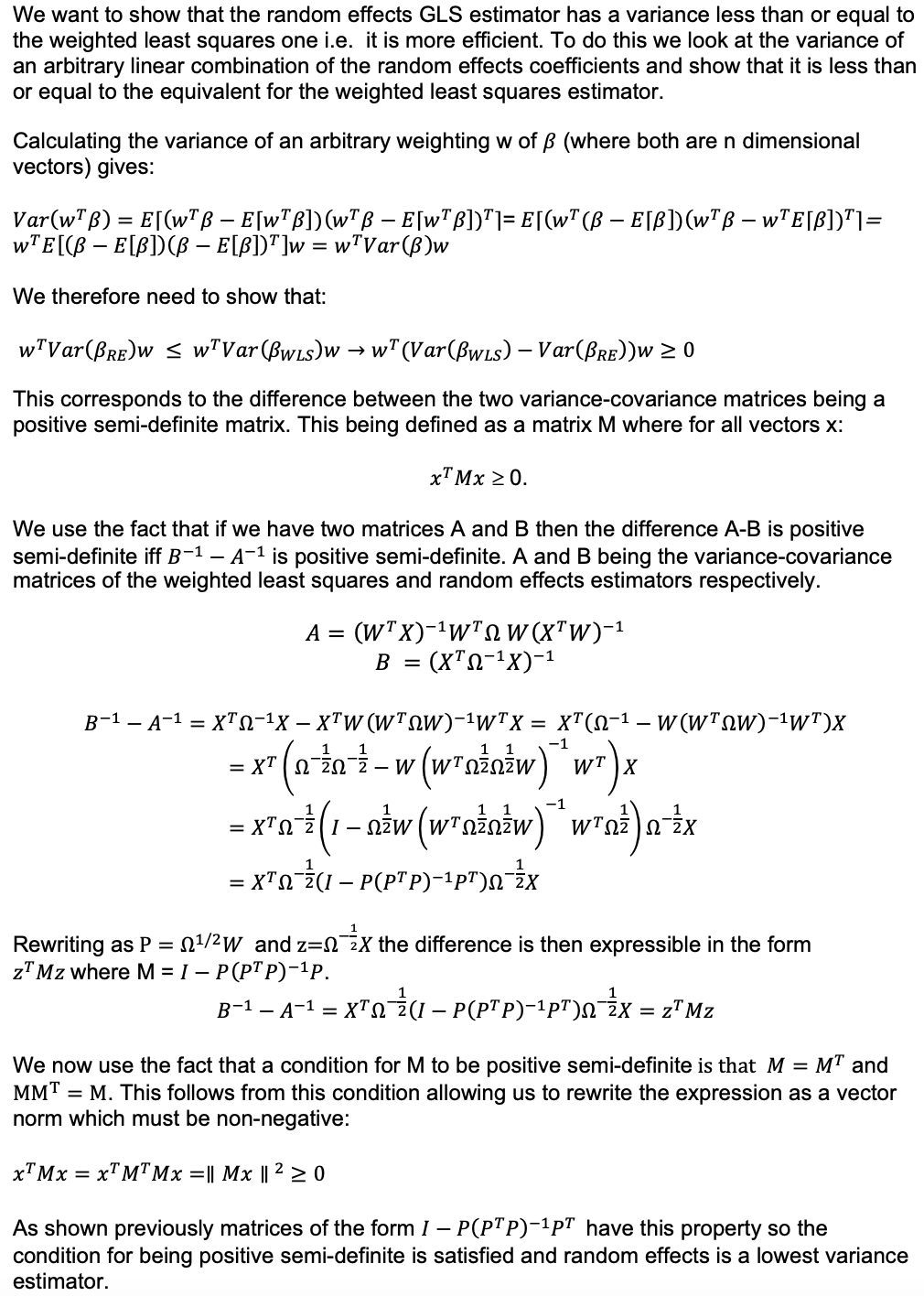
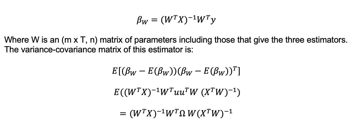 It can be shown (Appendix 3) that by looking at a weighted linear combination of the random effects coefficients (where we can isolate any coefficient by setting its weight to 1 and the others to 0) that the variance of these coefficients is always less than or equal to the equivalent variance of the weighted least squares estimator coefficients i.e. random effects gives us a minimum variance for this form of estimator.
3. Choosing between fixed and random effects
If the errors of the random effects model are uncorrelated with the explanatory variables then the random effects estimates of the coefficients should be better than a fixed effects approach as they will be unbiased and have lower variance.
However, it is often very plausible that unit specific factors which we do not have data on a) affect the dependent variable and b) will often be correlated with the explanatory variables biasing the coefficients estimated using random effects.
A standard test to distinguish the two alternatives is the Wu Haussman test which is based on the difference between the vector of estimated coefficients from fixed and random effects estimation and the two
corresponding variance-covariance matrices.
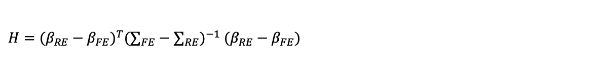
Where H is distributed as a Chi squared distribution with the degrees of freedom equal to the number of coefficients being estimated. The null hypothesis is that the random effects estimator is right. If we do not reject the null then this implies that there is a no difference between the random effects and the fixed effects estimator. This is an argument for using the lower variance random effects estimator. However, if fixed effects are substantively different that suggests random effects may be biased and we should use fixed effects instead.
If the random effects estimator passes the test, this may indicate it is a better estimator, but it is also consistent with there being insufficient variation in the explanatory variables to distinguish the two types of estimator.
Appendix 1: The OLS estimator is a combination of the between and within groups estimators
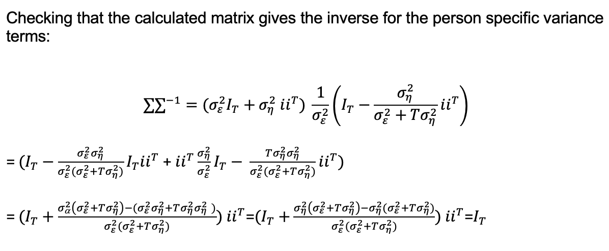
Appendix 2: Showing that we can invert the errors variance-covariance matrix
Appendix 3: Showing that the random effects estimator minimises variance