Centered: Notes on the ubiquitous topic of data normalisation

Crossrail Place Footbridge, October 2020

Data normalisation of variables in regressions i.e. transforming them to be mean zero with variance/standard deviation one (sometimes called standardisation) comes up frequently in work so it felt worth writing some notes on it.

Introduction

Regression variables are often on different scales e.g. if we are predicting shops’ revenue using inputs of the local population count in 1000s and their online rating between 1 and 5. In this context:

• the regression coefficients of the larger scale variables will generally be smaller as they have more variation. A comparison of the coefficients will suggest the variable on the smaller scale is more important, when in practice it may vary relatively little e.g online ratings can cluster at certain levels like four

• scales can be abitrary and affect coefficients of impact without affecting the fundamental reality such as when we express a variable in units of 100s rather than 000s

We therefore often standardise the data in regressions by subtracting each variable by its mean and dividing by its standard deviation. This puts them on a common scale where the values of the coefficients represent the effect of a standard deviation change in each of the variables helping compare what the effect of a typical change might be.

Applications of data normalisation:

There are several other applications of data normalisation, often with related motivations, such as in a:

• ridge regression to avoid it penalising the variables with the smallest scales and so the largest coefficients
• principal component (or clustering) analysis to prevent it prioritising dimensions on larger scales which account for more of the variance
• panel data regression to remove individual unit specific effects without using dummy variables
• Bayesian regression as the simulations of the posterior distribution converge better
• neural network’s inputs and in intermediate layers as this has been found to improve performance

Structure:

In these notes we work through the effects of normalisation’s two standard components where data is scaled by:

1. dividing by the standard deviation
2. subtracting the mean

This is done in the context of a linear model of the form: where we have k variables on n observations, y is a (n x 1) dependent variable vector, X an (n x k) matrix of explanatory variables, beta a (k x 1) vector of coefficients and eta a (n x 1) vector of random error terms.

I assume it is typically not possible to make general analytical statements on the effects of normalisation outside this basic linear case, or at least not easily.

1. Scaling the data by dividing by the standard deviation

Scaling the X variables

If we have a transform that is scaling the X variables by a variable specific factor e.g. dividing each variable by its standard deviation with n observations on k variables then this corresponds to multiplying the X matrix by a (k x k) diagonal matrix D where each diagonal element is the inverse of the variable’s standard deviation.

If a regression has a constant then the associated X column of ones will have zero variance and so normalisation by its standard deviation is not possible. As we usually want to estimate a constant we leave it unchanged in the transform with a corresponding diagonal 1 term. For example with 3 variables and a constant the transformation would be:

Applying the transformation matrix D we obtain the Ordinary Least Squares (OLS) estimator on the transformed variables XD as: Using the relationship of an inverse of a product of square matrices: and the fact that D is symmmetric we get:

Scaling the X variables changes the beta estimates by the inverse of the scaling factor. In the case of normalising the independent variables, this multiplies the associated beta estimates by their standard deviation. The constant is unchanged.

Geometrically as the transformation is a diagonal matrix it scales the basis vectors that the X data represents but does not change their orientation and the space spanned by them. As the original y vector remains unchanged the coefficients that define the corresponding projection of the y data we are trying to represent in this basis increase accordingly if the transform shrinks the size of the basis vectors as normalising by the standard deviation does.

Scaling the y variables

If we scale the y vector by a factor alpha e.g. dividing by the standard deviation of y then this scalar commutes with everything in the equation and we obtain:

Geometrically if the transformation is dividing by the standard deviation then the y vector shrinks and so correspondingly does the magnitude of the coefficients that are needed to describe it.

In general the scaling of the y variable is not done for ridge regression, but does happen in some Bayesian regression applications to assist convergence. If we have transformed the y data then obtaining the model’s predicted y values requires the transformation to be reversed to return the y values to their original scale. This is not necessary if only the X data is transformed.

The effect on the variance of the coefficients and test statistics

Calculating the effect on the variance of the betas: 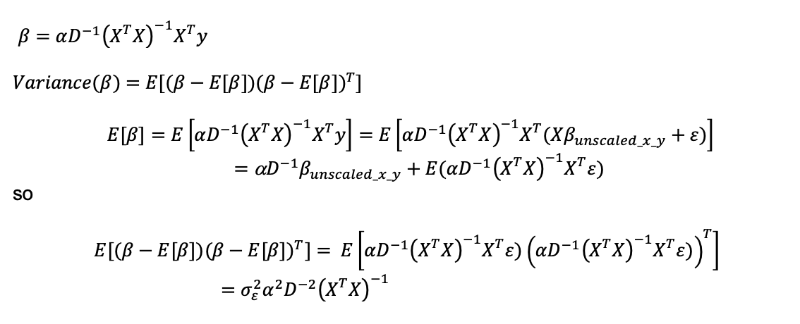The variance terms (which are the diagonal elements of the variance-covariance matrix) therefore change by the square of the scaling factors. This shows why we standardise by the standard deviation and not the variance. If we divide a variable by a scaling factor, then its variance is divided by the square of the scaling factor. When the scaling factor is the standard deviation the variance is then divided by the square of the standard deviation i.e. itself and is normalised to one.

The hypothesis tests are unchanged as in calculating the test statistics we normalise the estimated coefficients by the estimated standard deviation (the standard error) to allow us to use standard distributions. This removes the effect of the transformation on the test statistic. For example, specialising to one of the variables’ test statistics shows that the effects of the scaling factors cancel out.

2. Scaling the data by subtracting the mean

If we transform a matrix by subtracting the corresponding mean from each column then this is equivalent to the OLS regression of each variable on a vector of ones. The transformation on the X variables to subtract the mean is therefore:

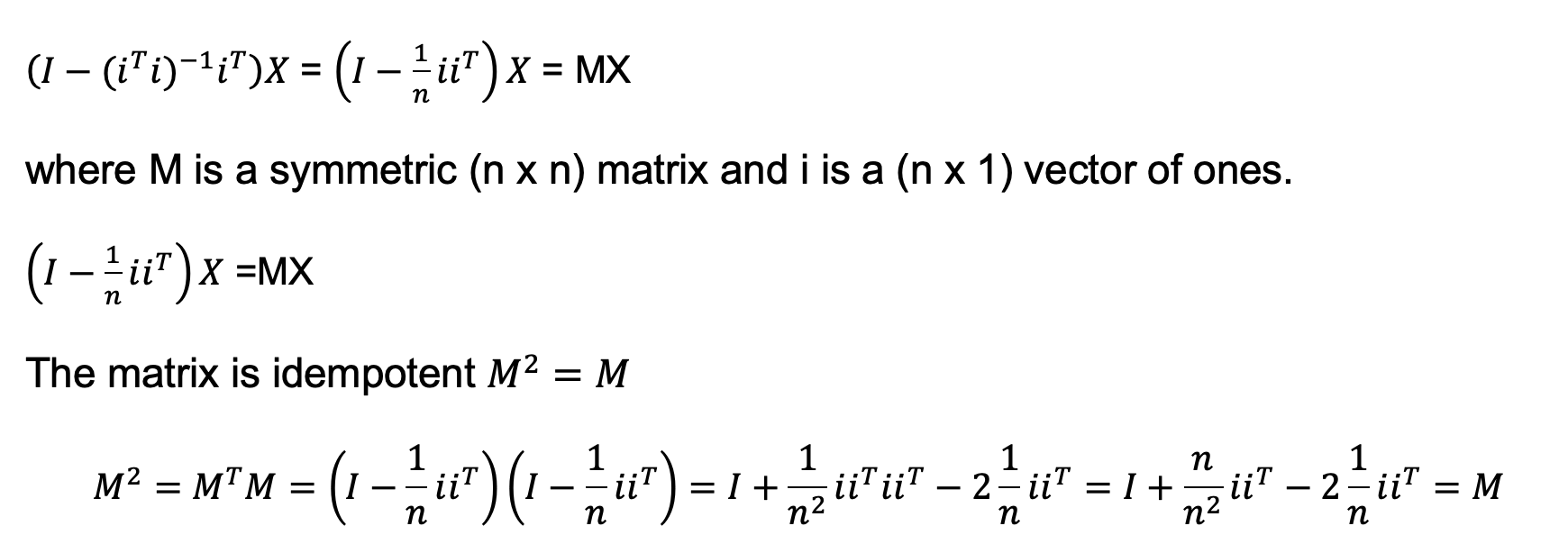If we transform the X variables we obtain the following OLS estimate:
If we transform both the X and the y variables we obtain the same beta estimates as if we ran the regression with just the X variables de-meaned:
This hides an important implication relating the values of the betas to the constant term in the regression. If we subtract the mean of the constant vector from itself then we get a vector of zeros. If this vector of zeros is included in the X matrix then it is not possible to calculate the inverse in the OLS estimation. This is because with a column of zeros there are an infinite number of values the constant can take so its value is indeterminate, matrix inversion fails and we cannot estimate the betas. Therefore the vector of ones representing the constant in the regression cannot be de-meaned and included in the regression, it has to remain unchanged.

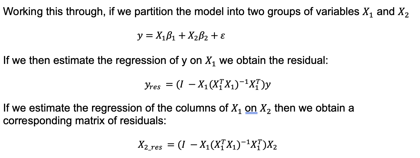
We unpack this by looking at the effect of subtracting the means in a more general way. The Frisch - Waugh - Lovell theorem says that in a linear regression if you:

1. regress the dependent variable y on a subset of the independent variables
2. regress the remaining independent variables on the first set
3. regress the residuals of the first regression on the residuals of the second regression

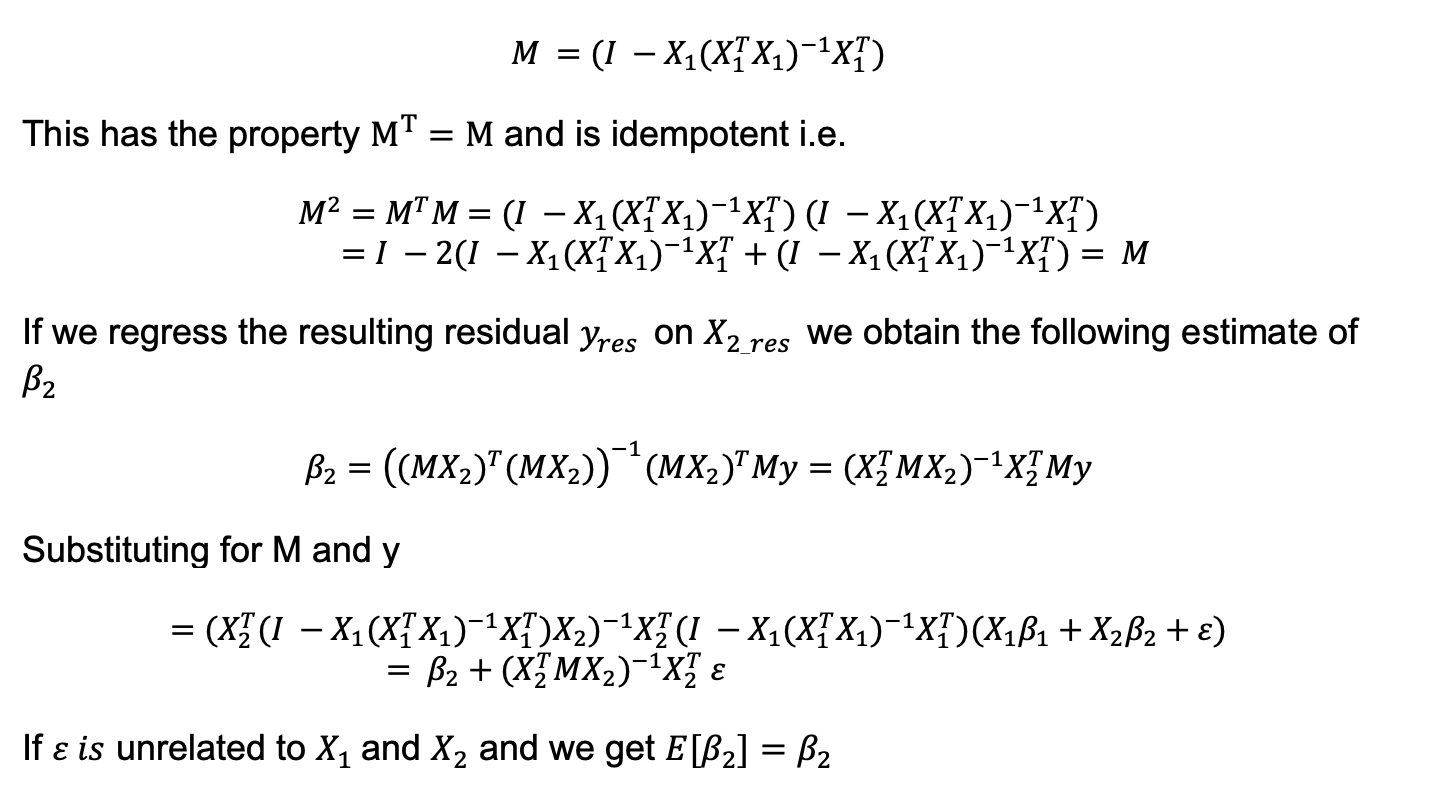
then the effects of the second set of independent variables are obtained. The projection matrix is:

Effects on the betas, variance and test statistics (and the constant)

Looking at the transformation in this way shows the implications of subtracting the means. When X_1 is the constant vector of ones then the regression of y and X_2 on it corresponds to the transformation of subtracting the means of the y and X variables. This gives the same estimate of beta_2 as we obtain without subtracting the means. The betas and variances of the non-constant variables are therefore unchanged by de-meaning and test statistics are as before. If we only de-mean the X variables (and not the y variables) this is also the case.

The intuition for why the coefficients of the non-constant variables are unchanged is that subtracting their means corresponds to moving the data points that represent them by a fixed vector (the vector of their means). The relative position of these points in the sample (i.e. the distances between them) does not change and so coefficients are unaffected. It is as if the data shifts, but does not change its shape. This is different from dividing by the standard deviation which does change the distance between points in the sample and hence the coefficients.

As the constant vector is not transformed that dimension’s position changes relative to the others. De-meaning therefore affects its coefficient leaving the others unchanged at their OLS values.

From the previous discussion it follows that in the transformed regression we do not need to include the constant to obtain unbiased estimates of the other variables’ coefficients. In a ridge regression the constant is typically not included in estimation as it cannot be normalised on a consistent basis and so will always have a different scale. However, in both cases we still need to estimate a constant if we want to obtain a predicted value of y. We therefore examine the effect of the transformations on the estimates of the constant. We could reverse the previous two stage regression analysis to obtain it, but instead use a different approach. Going back to the conditions the OLS estimator satisfies we can rewrite it as: If we partition the X variables and associated coefficients into two groups then this condition can be written as: Multiplying out and rearranging then we get the conditions: The coefficient groups can now be written in terms of the data and each other: Specialising to the case where X_1 is the constant vector i then beta_1 the associated estimated coefficient becomes: The constant coefficient estimate is therefore the average of the residuals between the y values and their predicted values from the other variables.

Effect on the constant of de-meaning both X and y variables: it becomes zero

Writing the OLS estimate for the constant coefficient with the y and X variables de-meaned using the M transformation (excluding the constant) and substituting in the estimate of beta_two it becomes: 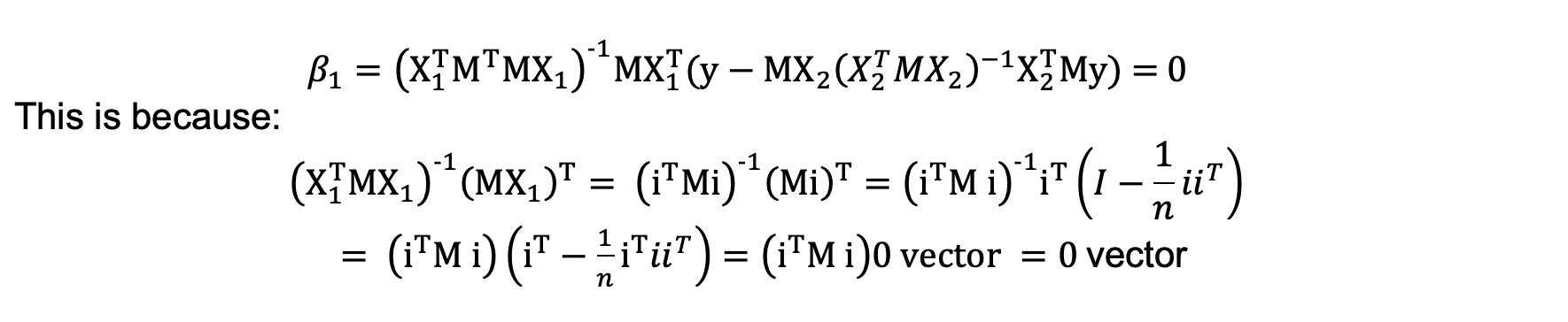With both X and y variables transformed the estimated constant will therefore be zero.

Effect on the constant when only the X variables are de-meaned: it becomes the average of y

If only the X data is de-meaned then the estimate of the intercept coefficient (beta_1) is the average of the y values. As we have not subtracted the mean of the y values it gets added back in to the constant.

The intuition behind this is that the constant coefficient on the untransformed data is the average value of the y variable minus the average values of the remaining X variables multiplied by their estimated coefficients. In subtracting the means from the X variables we are setting their average values to zero and so the constant coefficient is then the average of y. When we de-mean the y values the estimated constant i.e. the average of the transformed y values then becomes zero.

3. Both subtracting the mean and dividing by the standard deviation

Intuitively one should be able to subtract the mean and/or divide by the standard deviation and the effects are separate. If we apply the standard deviation normalisation D and the mean subtracting transform M to the X matrix excluding the constant then in the OLS estimator we see that we can factor out the effect of the standard deviation transformation making it independent of the mean subtraction transformation and vice versa. We can therefore combine both effects. Subtracting the X variables’ means while dividing by their standard deviations therefore multiplies the estimates of the variables coefficients by their standard deviations. As discussed the constant vector cannot be transformed and included in the OLS estimation as it would be zero under both transformations. When included untransformed its coefficient becomes the average of the y variable.

If the y variable is also transformed by subtracting its mean and dividing by its standard deviation then the constant estimate will always be 0 and the estimate of the slope coefficients will be divided by the standard deviation of the y variable. The hypothesis tests on the non-constant variables are unchanged when both X and y variables are transformed (the direct estimate of the constant excepted as it is zero).

References

Davidson and Mackinnon, ‘Econometric Theory and Methods’

Greene, ‘Econometric Analysis’