
Old Millfun, Shanghai, March 2026
Introduction
It felt useful to revisit some of the basics of the bias variance trade-off and ridge regression covering:
1. The relationship between a model’s forecast errors and its bias and variance
2. The trade-off between bias and variance
3. Ridge regression
4. An example of the bias and variance trade-off
The theory parts of these notes are based on Stanley H. Chan’s, ‘Introduction to Probability for Data Science’ and Wessel N. van Wieringen’s, ‘Lecture notes on ridge regression’
1. The relationship between a model’s forecast errors and its bias and variance
The starting point of the bias variance trade-off is that a model’s expected forecast performance (in terms of errors squared) can be decomposed into how much:
1. it deviates from the underlying true model (its bias squared)
2. it varies across its training data (its variance)
3. its residual errors vary
We assume that a value y is generated by a ‘true’ model f(x) with a random error term ε, where f(x) is a general function of x.

We do not know f(x) but can estimate a model of it f_hat. To assess how well this model will do we calculate its expected mean squared error:
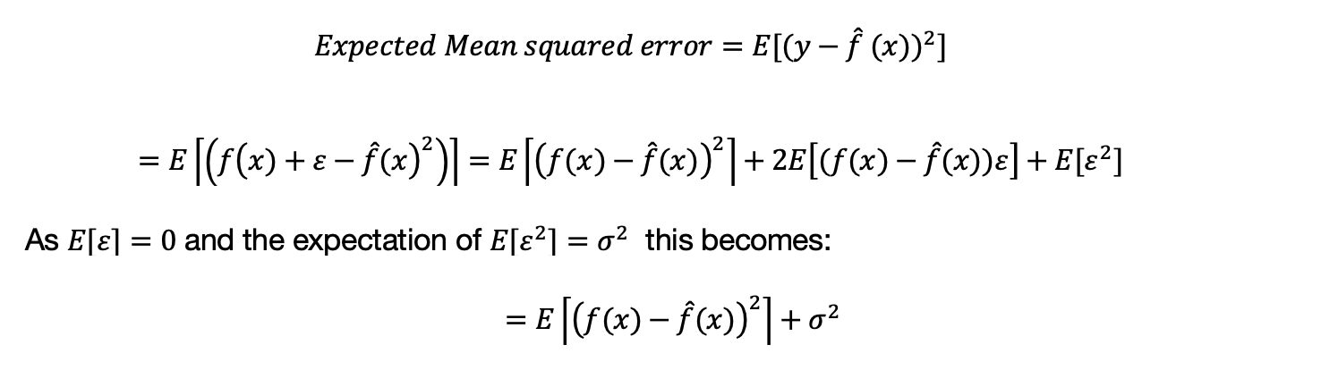 We want to rewrite this in terms of the bias and variance of the estimated model. To do this we use the trick of adding and subtracting the expectation of the estimated model to the equation. This allows us to express the expected mean squared errors in terms of the model’s bias squared, its variance and the variance of the error term along with a remainder term that we show has an expectation of zero.
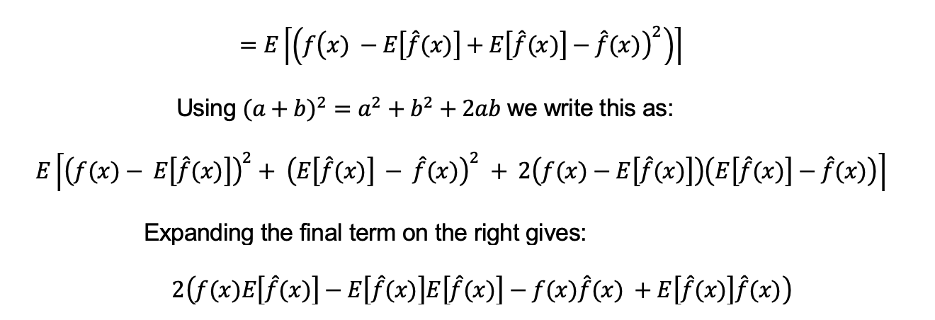 The expectation of the function f(x) is f(x) itself as it is non-stochastic.
 The expectation of an expectation returns the original expectation as that is a constant.
 The remaining terms therefore cancel to zero and we obtain the expected squared forecast error decomposed into three terms:

Although the function we use is quite general in a regression context, this decomposition is not true for classification problems, where the error function that is minimised typically a form of cross entropy that cannot be expressed in terms of separate model bias and variance terms.
2. The trade-off between bias and variance
The previous section has rewritten the model’s expected squared forecast errors in terms of its bias and variance. It has not shown any trade-off between bias and variance. It suggests increasing a model’s forecast performance by reducing its:
- bias
- variance
However, the bias and variance can be related to each other which makes it harder to reduce both simultaneously.
In general one would expect a simple model to have a lower variance across training samples as it has fewer parameters and so there is less scope for it to be affected by new training data. For example a function that was a constant independent of x would have no variance and only the bias term would remain. If the reality is that the y values are a complicated function of x then a simple model will not be able to fit the true model and be more likely to be biased.
If we had a more complicated model e.g. a model with more variables or more interactions between variables then one might expect there to be less bias. However, even if the model was unbiased there will still be variance caused by its outputs being sensitive to the data it is trained on. A model with more parameters is therefore likely to have a higher variance.
3. Ridge regression
A way to address the bias variance trade-off is ridge regression which follows the strategy of reducing the model’s variance to improve forecast performance.
We assume we have a linear model written in matrix form where y is a (n x 1) dependent variable vector, X an (n x k) matrix of explanatory variables, β a (k x 1) vector of coefficients and ε a (n x 1) vector of random error terms.
 We can extend the standard optimisation of choosing β to minimise the total of the sum of squared errors to minimising the total of this and the sum of the squared coefficient values multiplied by a regularisation parameter λ. The latter penalises choosing larger model coefficients reducing the model’s variance and so hopefully improving forecast performance.
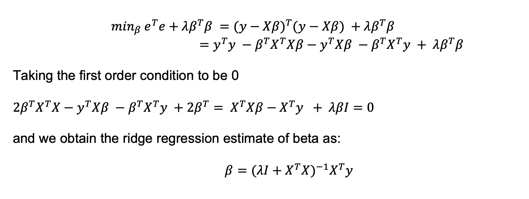 This is a generalisation of the Ordinary Least Squares (OLS) solution which is obtained when lambda is equal to zero. As the OLS estimator is an unbiased estimator, we know that the ridge regression which deviates from this is a biased estimator of β. As larger coefficient values of β are penalised the regulator term pushes the coefficient estimates towards 0.
Calculating the variance of the estimated coefficients:
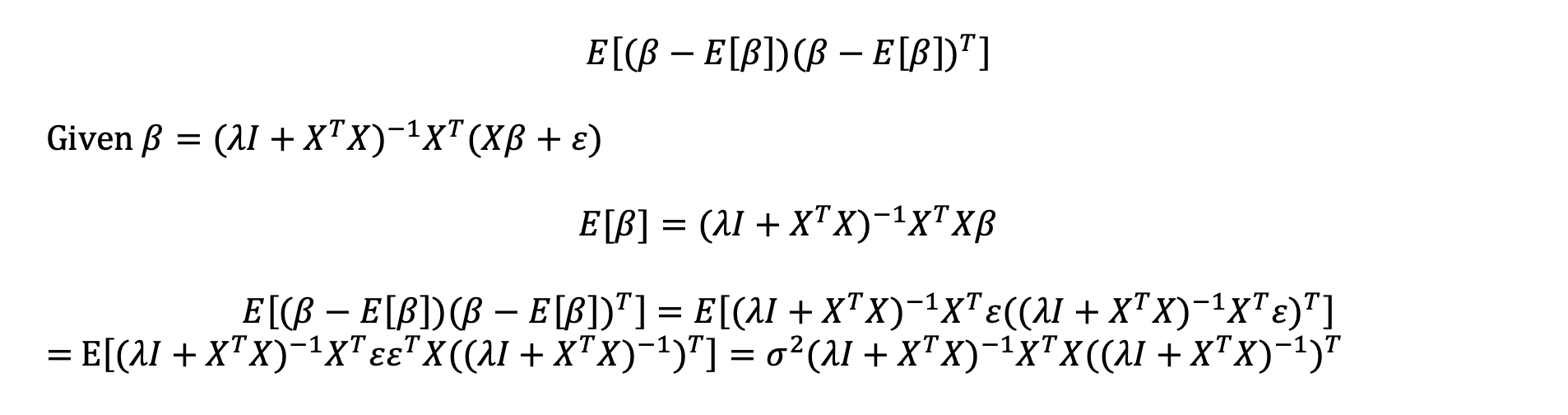 It is possible to show (see the Appendix) that ridge regression, while biased, has a lower variance than a normal OLS regression.
For a given data set it is possible to estimate what an optimal value of lambda might be using cross-validation over hold-out samples. However there is no general theory that will give an optimal lambda. There is also no guarantee that the reducing the forecast’s variance at the expense of the bias will improve its performance.
The connection to Bayesian estimation and Lasso
Another perspective on ridge regression is that we can obtain it by imposing certain restrictions on the priors of a Bayesian model. If we estimate a Bayesian version of the standard linear model where the likelihood and prior are normally distributed and then solve out for the values of the beta coefficients that maximises the resulting posterior distribution we get the following estimate of the betas:
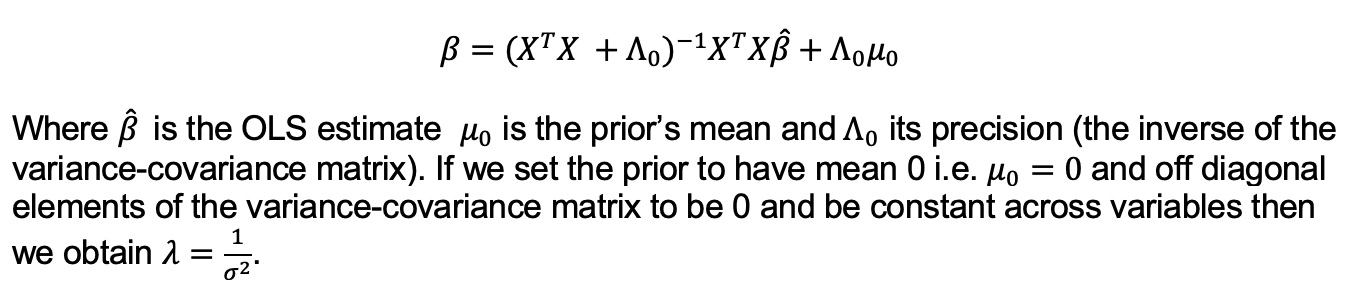 Ridge regression is therefore equivalent to a Bayesian regression with a prior of 0 slope coefficients and homoscedasticity across variables.
In the case of a Lasso (Least absolute shrinkage and selection operator) regression where we have the sum of the betas as the regulator term:
 then specific individual coefficient estimates among the variables are set to zero (unlike ridge regression this does not have an analytical solution). Lasso has the advantage compared to ridge that it will produce a simpler and more interpretable model by selecting specific variables for the model among the original set, although this does not necessarily improve the forecast accuracy.
4. An example of the bias and variance trade-off
To make the bias and variance trade-off more concrete we write a Python class BiasVariance that generates a simple example.
The class has the following methods:
-
_create_test_train_dataCreates test and train datasets. As our ground truth we specify a seventh order polynomialwiggly_polynomialto which random noise is added to produce the test and train datasets. We generate the corresponding y values at 51 evenly spaced x values between 0 and 100. -
_create_estimate_regressionEstimates a regression on this data where we can specify the order of the estimated polynomial model and the value of the regularisation parameter (giving a normal regression if lambda = 0). -
_calculate_errorsCalculates the model’s:
• errors squared
• bias squared
• variance -
_chart_itCharts the different values of the regression across the training sample along with the underlying true model.
In the method _calculate_errors we approximate the expectations in the bias variance relationship by averages over the test and training samples. In the expected:
• sum of squared errors for each x value we calculate the sum of squared errors for each test sample relative to the predictions from the training sample. We then average that over the test samples at a given x value and then average the resulting values over the x values.
• bias squared for each x value we calculate the average of the predictions over the training samples. We square the difference between the true model value and the average at each of the x points. This value is the same across all the training samples so we calculate it once rather than average it over the training samples which would give exactly the same number. We then average the resulting squared deviation of the average model across the x values.
• variance squared for each x value we calculate the difference between a forecast from the training sample and the average forecast over the training samples and square that. We then average that across the training samples at each x value and then average the resulting values over the x values.
import numpy as np
from numpy.polynomial import Polynomial
import pandas as pd
from sklearn.linear_model import Ridge
from pprint import pprint

import matplotlib
matplotlib.use("Agg")
import matplotlib.pyplot as plt
from matplotlib.ticker import FuncFormatter
import matplotlib.ticker as ticker


def wiggly_polynomial(x):
    z = (x - 50) / 50

    return 30 * z ** 7 - 5 * z ** 5 + 5 * z ** 3 - 4 * z


class BiasVariance:
    """A class that demonstrates the bias variance trade-off
    Args:
        truth_func: The underlying true function that generates the data.
        train_polynomial_degree (int): The degree of the polynomial used to fit the training data.
        sample_size (int): The number of training and test samples to generate
    Methods:
        _create_test_train_data(self): Creates the test and training datasets based on the true function.
        _create_estimate_ridge_regression(self, lambda_param): Estimates the model using ridge regression with the specified lambda parameter.
        _calculate_errors(self, model_forecast): Calculates the bias, variance, and sum of squared errors from the forecast.
        _chart_it(self): Charts the estimated regressions on training data and the ground truth
    """

    def __init__(self, truth_func, train_polynomial_degree, sample_size):
        """Class that illustrates the BiasVariance trade-off"""
        # The function that we pass as the ground truth
        self.truth_func = truth_func
        # The x values we are evaluating the function over
        self.x_inputs = np.linspace(0, 100, 51)
        # Calculate the true function values given the x_inputs
        self.truth_func_values = self.truth_func(self.x_inputs)
        # The order of the polynomial we are trying to fit
        self.poly_train_deg = train_polynomial_degree
        # The value of the lambda parameter
        self.lambda_param = None
        # The number of test and training samples we generate. For simplicity we assume these have the same sample size.
        self.sample = sample_size
        self.train_data = None
        self.test_data = None
        # collection of error metrics
        self.error_metrics = {}

    def _create_test_train_data(self):
        """Creates test and train datasets based off an underlying true model"""
        # Creates two sets of noise for the test and train data with mean 0 and standard deviation 10
        samples = np.random.normal(size=(self.sample, 51), scale=10)
        samples2 = np.random.normal(size=(self.sample, 51), scale=10)
        # Adds the random noise to the true model to create the test and train datasets
        self.test_data = self.truth_func_values + samples
        self.train_data = self.truth_func_values + samples2
        return self

    def _create_estimate_ridge_regression(self, lambda_param):
        """Creates an estimated model predicting y from the training data"""
        # initialises the ridge regression
        self.lambda_param = lambda_param
        ridge = Ridge(lambda_param, fit_intercept=True)
        # Create a matrix with multiple variables 1, x, x^2, x^3 etc in ascending order for the polynomial we specify the degree of
        # We drop the first column as this is this will be fitted separately
        V = np.vander(self.x_inputs, increasing=True, N=self.poly_train_deg + 1)[:, 1:]
        # Fit the ridge regression on the training data
        ridge.fit(V, self.train_data.T)
        # Extracts the estimated coefficients and intercept and make a prediction
        coeffs = ridge.coef_
        intercept = ridge.intercept_
        coeff_pred = V @ coeffs.T
        self.estimated_regression_ridge = intercept + coeff_pred
        return self.estimated_regression_ridge

    def _calculate_errors(self, model_forecast):
        """Calculate the bias, variance, and sum of squared errors from the input forecast"""
        # Average the model forecasts across the training samples (axis=1) giving an average forecast for each of the x values (axis1)
        self.mean = model_forecast.mean(axis=1)

        # Average the squared errors across the test and training datasets at each x value, average over the different x values
        self.sse = ((model_forecast - self.test_data.T) ** 2).mean(axis=1).mean(axis=0)

        # Calculate the variance of the model across the training datasets at each x value, average over the different x values
        # , None is used to broadcast the mean across the different training samples for each x value
        self.estimator_var = (
            ((model_forecast - self.mean[:, None]) ** 2).mean(axis=1).mean(axis=0)
        )

        # Calculate the bias squared of the model as the:
        # ground truth minus the average of the model forecasts from the training datasets, average over the different x values
        self.estimator_bias_sq = ((self.truth_func_values - self.mean) ** 2).mean(
            axis=0
        )

        # Return the metrics as a dictionary
        self.error_metrics = {
            "sum of errors squared": self.sse.round(1),
            "bias squared": self.estimator_bias_sq.round(1),
            "variance": self.estimator_var.round(1),
        }
        return self

    def _chart_it(self):
        """charts the estimated regressions on training data and the ground truth"""
        ax = plt.gca()
        x = self.x_inputs
        # plot the different regressions estimated from the training data
        plt.plot(x, self.estimated_regression_ridge, alpha=0.2)
        # plot the average model output from the training data
        plt.plot(x, self.mean, alpha=1, color="black")
        # plot the ground truth as a blue curve
        plt.plot(x, self.truth_func_values, color="blue")
        ax.yaxis.set_major_formatter(ticker.StrMethodFormatter("{x:,.2f}"))
        plt.xlabel("x")
        plt.ylabel("y")
        plt.title(
            f"Estimated polynomial of order {self.poly_train_deg}, lambda {self.lambda_param}, sample size {self.sample}"
        )
        filepath = f"plot_{self.poly_train_deg}_{self.lambda_param}_{self.sample}.png"
        plt.savefig(filepath)
        plt.close()
        return self
To apply the class
# Creates an instance of the class
BV_example = BiasVariance(
    truth_func=wiggly_polynomial, train_polynomial_degree=10, sample_size=50
)
# Creates the test and training data
BV_example._create_test_train_data()
# Estimates a ridge regression with a given lambda parameter
BV_example._create_estimate_ridge_regression(lambda_param=1)
# Calculates the errors associated with a given estimated metric
BV_example._calculate_errors(BV_example.estimated_regression_ridge)
# Charts the regressions from the training data, their average and the ground truth
BV_example._chart_it()
# Prints the error metrics
print(BV_example.error_metrics)
The chart below shows a series of curves estimated using OLS on 50 random training samples. The blue curve shows the underlying true model that in combination with the random noise is generating the data. The black curve shows the average of the model forecasts across the training data. The spread of the lighter individual training run curves around this gives a sense of the model variance.
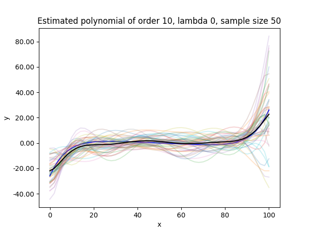 The variance of the errors added to any given point is 100 and so when added to the model’s bias squared and variance we approximate the sum of errors squared relationship in the bias variance decomposition.
{'sum of errors squared': 120.4, 'bias squared': 0.3, 'variance': 21.8}
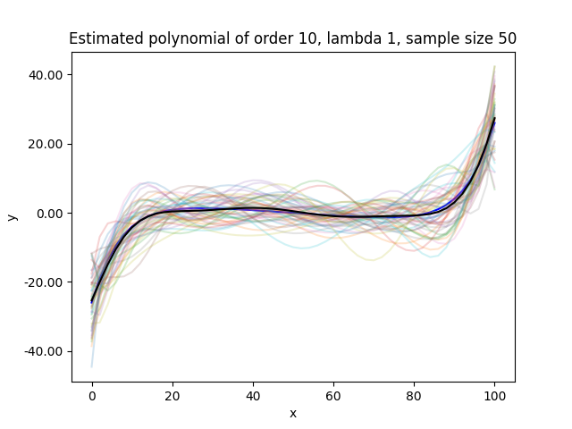
If we then apply the ridge regression penalising the variation setting lambda to one then the curves estimated from the different training samples vary less.
 .
.
{'sum of errors squared': 119.2, 'bias squared': 0.1, 'variance': 20.6}
In the example we get a slight improvement on the forecast with both the bias and the variance reduced from running the ridge regression. In our case as we are fitting a model that is more complicated than the ground truth the normal OLS estimate is also biased.
References
Stanley H. Chan, ‘Introduction to Probability for Data Science’
Efron and Hastie, ‘Computer Age statistical inference’
Kevin P. Murphy, ‘Machine Learning a Probabilistic Perspective’
Wessel N. van Wieringen, ‘Lecture notes on ridge regression’
Appendix 1: comparing the variance of the OLS and ridge regressions
We want to show that:
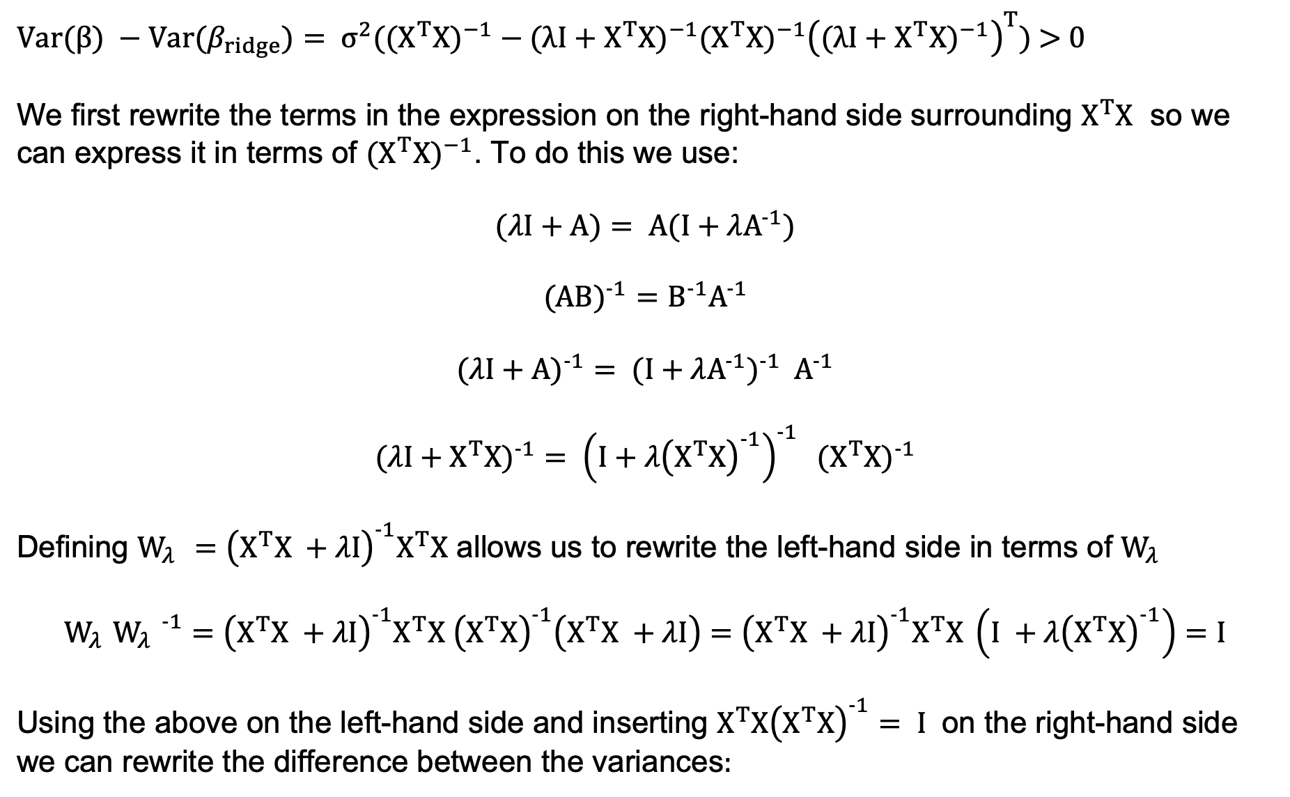 To do this we need to show that the difference between the variance-covariance matrix of the OLS and ridge regressions is positive semi-definite where w is a non-zero vector:
 If this is the case we can choose w to isolate the individual coefficient variance terms and thus show the OLS variance is larger.
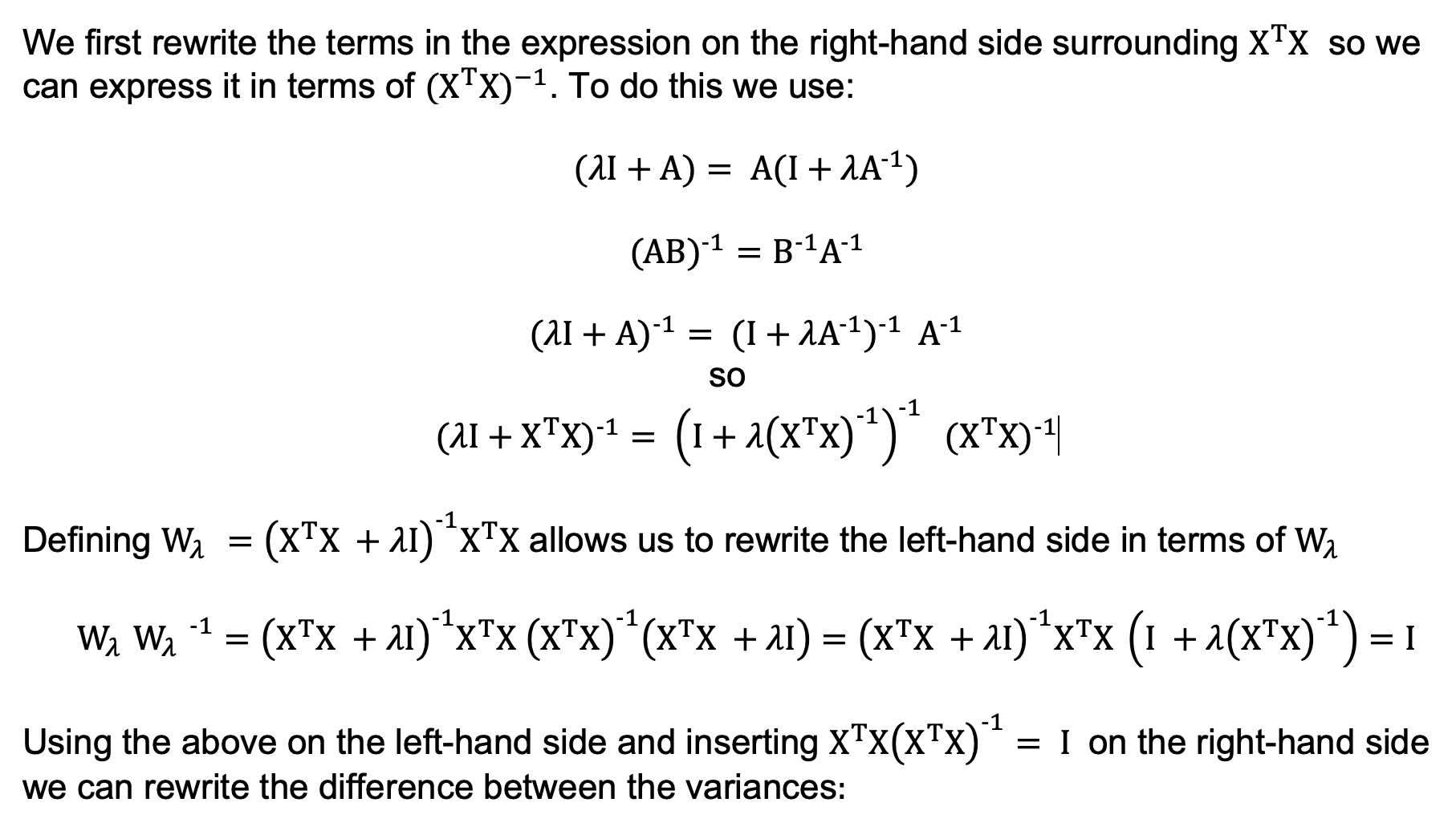
 Expanding the term in the central bracket gives:
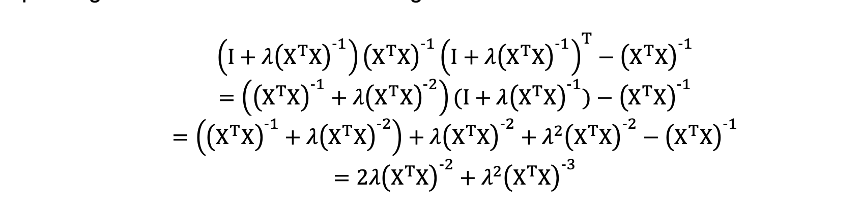 Multiplying by the terms in the outer brackets:
 And we reduce the expression to:
 The variance-covariance matrices in the expression are always positive semi-definite. This is because if we have a vector of random variables like the beta and we calculate the variance of weighted sum of these variables, then this expression can be written in terms of the positive semi-definite condition where the matrix it applies to is the variance-covariance matrix of the random variables. The positive semi-definite condition is satisfied as the variance of the weighted sum must be a scaler with variance greater than or equal to zero.
 The remaining diagonal lambda terms obtained after rearranging are positive definite leading to the expression overall being positive definite if lambda is greater than 0. The ridge regression therefore has a lower variance than the standard OLS estimator.