Ilke Sahin’s ‘Water Canals (Aquaducts)’ at Goldsmiths degree show 2024
This note reviews some basic aspects of Bayesian inference to refresh my knowledge of it and some of the probability distributions it often uses.
1. Finding the most probable parameters given the data using Bayes’ theorem
We want to find the best hypothesis or model parameter(s) that describes the data. Bayes’ theorem allows us to write down a general formula for this:

This is called the posterior distribution. It consists of a prior, a likelihood, and a marginal likelihood (sometimes called the evidence). The prior gives the assumed probability distribution of model parameters/hypotheses (here represented by theta) before any data. This can reflect pre-existing beliefs and/or logical/physical constraints. The likelihood gives the probability of the observed data given a set of parameter values/hypotheses. The marginal likelihood is the probability of the data given all possible hypotheses/values the model parameters might take (here represented by alpha).
The starting point in a Bayesian approach is that there is assumed to be an uncertainty about the model parameters which we capture with a prior distribution and then update the posterior as new data comes in. By contrast, in a frequentist approach, there are assumed to be true underlying model parameters and the data sampled from the model generates uncertainty in our parameter estimates. We capture this uncertainty in a frequentist approach in the sampling distribution of the estimates.
If a parameter or hypothesis can only take discrete values e.g. does a photo (the data) contain person A (hypothesis 1) or does it not (hypothesis 2). Then the Bayesian formula looks like the below where the marginal likelihood is a sum over all possible states:

If the parameter can take an infinite number of values, for example a parameter specifying a distribution, then the denominator becomes an integral:

We often want to find the value of theta that maximises the posterior and so is the most probable value given the data. The marginal likelihood does not depend on theta as we integrate over all possible values of it. It therefore represents a normalisation constant which will not affect the optimal value of theta. As a result a lot of Bayesian statistics is about evaluating the likelihood*prior to estimate the optimal parameter, rather than the full posterior. For a given model the marginal likelihood is fixed, but it can vary between models with different numbers and types of parameters and so different scope to explain the data. It therefore has a role in choosing between models.
To make the posterior more concrete we now work through a simple example of calculating it based on a Poisson likelihood and a Gamma prior distribution. These functional forms allow the posterior to be completely solved analytically. This is often not possible and techniques like Markov Chain Monte Carlo (MCMC) have to be used to estimate the posterior.
2. The Likelihood: A Poisson distribution
The Poisson distribution gives the probability that a certain number of types of events x occur in an interval (such as a time period or number of discrete events). Its probability distribution below has both a mean and variance of lambda.

As a probability distribution when summed from x=0 to infinity it adds up to 1.

Calculating the expected value:

The Poisson is the limit of the Binomial distribution as sample sizes get large. The Binomial is the distribution of x outcomes from n trials where there are two possible states e.g. how many heads from n coin tosses. Where p+q=1 and lambda=p*n it tends to the Poisson as n increases.

Assuming different observations are independent of each other then the likelihood function is the product of the probabilities (i.e. the Poisson distributions) for each observed value. The likelihood of the data then becomes:

3. The Prior: A Gamma distribution
Having got an expression for the likelihood of lambda given the data we now examine a prior for lambda. A standard prior for a variable with a Poisson likelihood distribution is the Gamma distribution shown below. As the Gamma distribution is defined from 0 to infinity it gives a probability distribution over the values lambda could take (which cannot be negative). The distribution is specified by two parameters alpha and beta.

Where Gamma(alpha) in the denominator is the Gamma function which generalises the factorial function ! to the real numbers. It has the functional form:

That the Gamma distribution integrates to 1 can be seen by integrating it over x between 0 and infinity.

which is the same as the Gamma function in the denominator, so the whole thing integrates to 1.
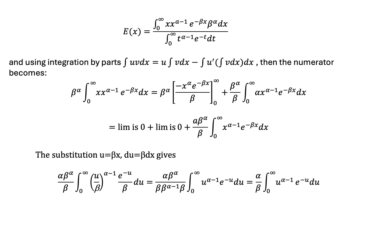
The mean of the Gamma distribution is alpha/beta. Taking the expectation of the distribution:

Normalising by the Gamma function in the denominator then cancels the Gamma function in the numerator giving E(x)=α/β
In our example the prior is specified by two parameters alpha0 and beta0 and so has the form:

4. Calculating the Posterior distribution analytically
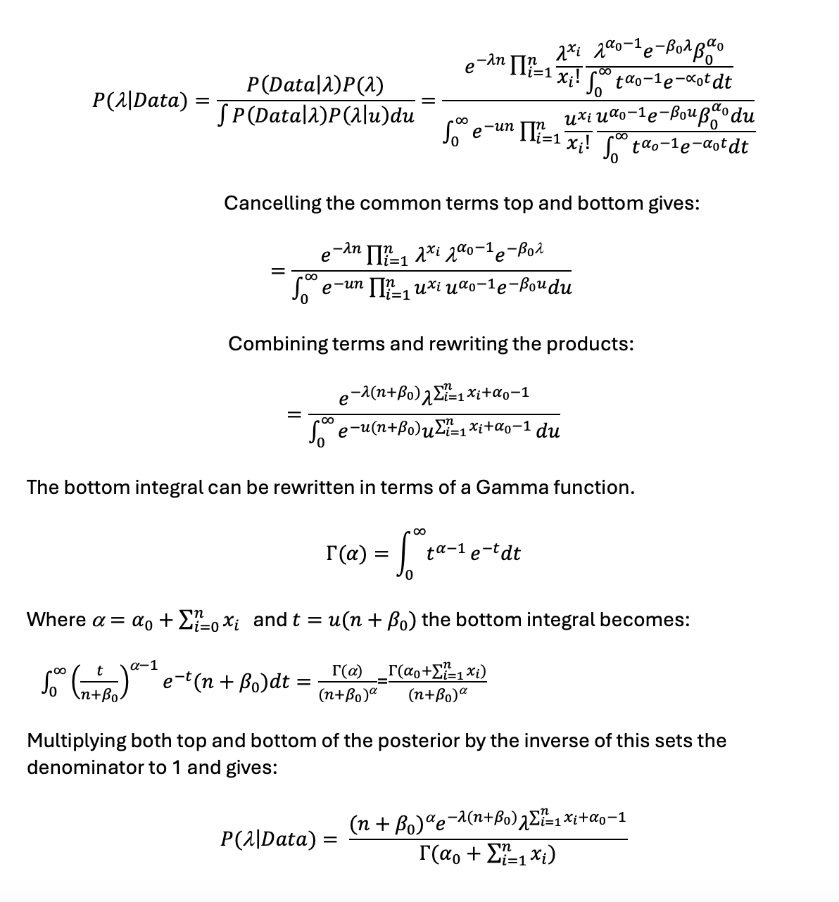
With this prior and likelihood, we can substitute into Bayes’ formula and directly calculate the probability of the lambda parameter given the data. In the denominator, with the marginal likelihood, we integrate over all values of lambda (here using the variable u) to give the probability of the data conditional on all possible values of lambda.
A Gamma prior distribution and a Poisson likelihood generates a posterior that is itself a Gamma distribution.

Now we can see that the posterior also has a Gamma distribution just like the prior, updating the posterior with new data while maintaining the same functional form. If we have no data i.e. xi=0 and n=0 we get back the original prior:

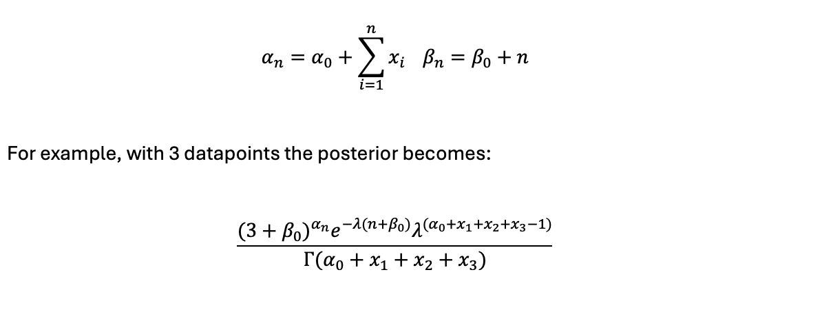
As as we get more datapoints we just update this formula. The original alpha parameter in the posterior is increased by the sum of the subsequent observed datapoints. The beta parameter is increased by the number of new datapoints i.e.

When a prior combined with a given likelihood leads to a posterior distribution of the same functional form it is known as a conjugate prior. Another example of a conjugate prior is that a Normal prior and a Normal likelihood gives a posterior Normal distribution. For a Binomial likelihood and a Beta prior distribution the posterior will also have a Beta distribution.
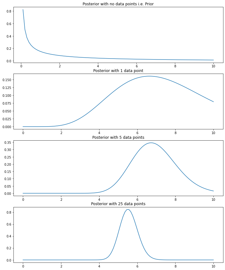
We can see from the simulated example below that as we add more data the posterior moves away from the prior and increasingly reflects the data.
import numpy as np
import matplotlib.pyplot as plot
from scipy.special import gamma

def posterior(lambda_val, alpha, beta, data):
    """function that gives the values of the gamma posterior for different values of alpha, beta and data"""

    count_no = len(data)
    sum_val = sum(data)
    new_beta = beta + count_no
    new_alpha = alpha + sum_val

    numerator = (
        (new_beta ** new_alpha)
        * np.exp(-lambda_val * new_beta)
        * (lambda_val ** (new_alpha - 1))
    )
    denominator = gamma(new_alpha)

    val = numerator / denominator

    return val

# Generate values to evaluate posterior
x_vals = np.linspace(0, 10, 100)

# Generate chart values
chart_0 = posterior(l_vals, 0.3, 0.1, [])
chart_1 = posterior(l_vals, 0.3, 0.1, list(np.random.poisson(6, 1)))
chart_2 = posterior(l_vals, 0.3, 0.1, list(np.random.poisson(6, 5)))
chart_3 = posterior(l_vals, 0.3, 0.1, list(np.random.poisson(6, 25)))

# Generate chart
fig, axs = plot.subplots(4, figsize=(12, 15))

axs[0].plot(x_vals, chart_0)
axs[0].set_title("Posterior with no data points i.e. Prior")

axs[1].plot(x_vals, chart_1)
axs[1].set_title("Posterior with 1 data point")

axs[2].plot(x_vals, chart_2)
axs[2].set_title("Posterior with 5 data points")

axs[3].plot(x_vals, chart_3)
axs[3].set_title("Posterior with 25 data points")

References:
Donovan, T. and Mickey, R. ‘Bayesian Statistics for Beginners’
Efron, B. and Hastie, T., ‘Computer Age Statistical Inference’
Williams, D., ‘A course in Probability and Statistics’
